This walkthrough follows the original examples/3_channel_example_walkthrough.ipynb notebook. Download the notebook or Python script. The figures show saved results from this example dataset. Run the notebook to reproduce the analysis.
Three-channel walkthrough: DAPI and GFP-DnaN objects
Each field contains phase contrast (C1), DAPI (C2, DNA/nucleoid), and GFP-DnaN (C3, replication-associated puncta). We segment cells, inspect masks and meshes, curate with the supplied SVM, detect C3 objects without channel alignment, and extract per-cell features.
Run the cells from top to bottom. All images, masks, models, and outputs stay in the three-channel example folder. Set RUN_DIR in the first code cell if you moved that folder. The supplied masks let you set RUN_SEGMENTATION = False; masks from other tools also work when the background is 0 and distinct cells are labeled consecutively 1 through N. Omnipose uses a GPU when available and otherwise runs on CPU. See the installation guide for installation.
from pathlib import Path
import sys
import torch
import pandas as pd
import matplotlib.pyplot as plt
from IPython.display import display

# Import BactoScoop
# Import the package installed in this notebook kernel.
import bactoscoop
import bactoscoop.plot as bplt

# Point to the folder containing C1-C3 TIFFs, masks/, and the SVM model.
# Locate the downloaded examples; keep the supplied inputs unchanged.
import os
import shutil
from datetime import datetime

EXAMPLES_DIR = os.environ.get("BACTOSCOOP_EXAMPLES_DIR")
candidates = ([Path(EXAMPLES_DIR)] if EXAMPLES_DIR else
              [candidate for base in (Path.cwd(), *Path.cwd().parents)
               for candidate in (base / "examples", base)])
SOURCE_DIR = next((base / "3_channel_example" for base in candidates
                   if (base / "3_channel_example").is_dir()), None)
if SOURCE_DIR is None:
    raise FileNotFoundError("Open this notebook from the downloaded examples folder, "
                            "or set BACTOSCOOP_EXAMPLES_DIR to that folder.")
RUN_DIR = Path.home() / "bactoscoop_runs" / datetime.now().strftime("%Y%m%d_%H%M%S_%f") / "3_channel_example"
shutil.copytree(SOURCE_DIR, RUN_DIR)
MODEL_PATH = RUN_DIR / "DnaN_Timecourse.pkl"
RUN_SEGMENTATION = False  # Reuse supplied masks; set True for fresh Omnipose inference.
PIXEL_SIZE_UM = 0.065  # Replace with your microscope calibration.
PHASE_CHANNEL, DAPI, GFP_DNAN = "C1", "C2", "C3"
CHANNEL_LABELS = {"C1": "Phase contrast", "C2": "DAPI", "C3": "GFP-DnaN"}

if not RUN_DIR.is_dir():
    raise FileNotFoundError(f"Example folder not found: {RUN_DIR}")
if not MODEL_PATH.is_file():
    raise FileNotFoundError(f"SVM model not found: {MODEL_PATH}")
(RUN_DIR / "masks").mkdir(exist_ok=True)
FIELD_IDS = bplt.list_field_ids(RUN_DIR, phase_channel=PHASE_CHANNEL)
print("Fields:", FIELD_IDS)
print("Image and output folder:", RUN_DIR)
print("CUDA available:", torch.cuda.is_available(), "(CPU is used when False)")
1. Inspect the input channels
The field name is the shared part of each filename before _C1, _C2, or _C3. Display contrast is adjusted for the overview; measurements use the original image values. DAPI is cyan and GFP-DnaN is green.
fig = bplt.plot_multichannel_overview(RUN_DIR, FIELD_IDS[1], CHANNEL_LABELS, )
display(fig)
plt.close(fig)
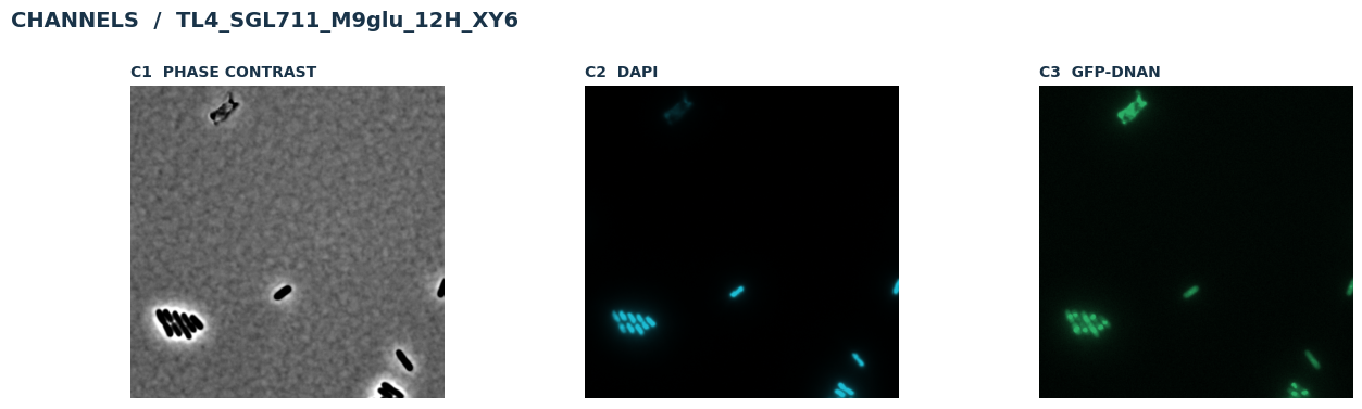
1. Inspect the input channels. Saved notebook output from 3_channel_example; display settings are illustrative.
2. Segment and review
RUN_SEGMENTATION=True segments the C1 phase images with Omnipose. mask_thresh adjusts the mask boundary and minsize removes small segments. If you set the flag to False, the supplied masks in masks/ are loaded instead. The review compares phase with mask outlines in the same crop. Change the field, label, center, or crop size in the review cell to inspect another region; a 700-pixel crop shows many cells, while about 150-250 pixels is useful for a close check.
collection = bactoscoop.ImageCollection(str(RUN_DIR), px=PIXEL_SIZE_UM)
collection.load_phase_images(phase_channel=PHASE_CHANNEL)
if RUN_SEGMENTATION:
    ok = collection.segment_images(
        mask_thresh=1, minsize=100, n=range(len(collection.images)),
        model_name="bact_phase_omni",
    )
    if not ok:
        raise RuntimeError(collection.processing_summary())
collection.create_image_objects(phase_channel=PHASE_CHANNEL)

# Change these values and rerun this cell to inspect another field or label.
SEGMENTATION_FIELD = FIELD_IDS[0]
SEGMENTATION_LABEL = None  # Integer mask label, or None for a central cell.
SEGMENTATION_CENTER = None  # Optional (row, column), used when label is None.
SEGMENTATION_CROP_PX = 700
review_image = next(image for image in collection.image_objects
                    if image.image_name.rsplit("_", 1)[0] == SEGMENTATION_FIELD)
fig = bplt.plot_segmentation_review(
    [review_image], crop_size=SEGMENTATION_CROP_PX,
    mask_label=SEGMENTATION_LABEL, center=SEGMENTATION_CENTER,
)
display(fig)
plt.close(fig)
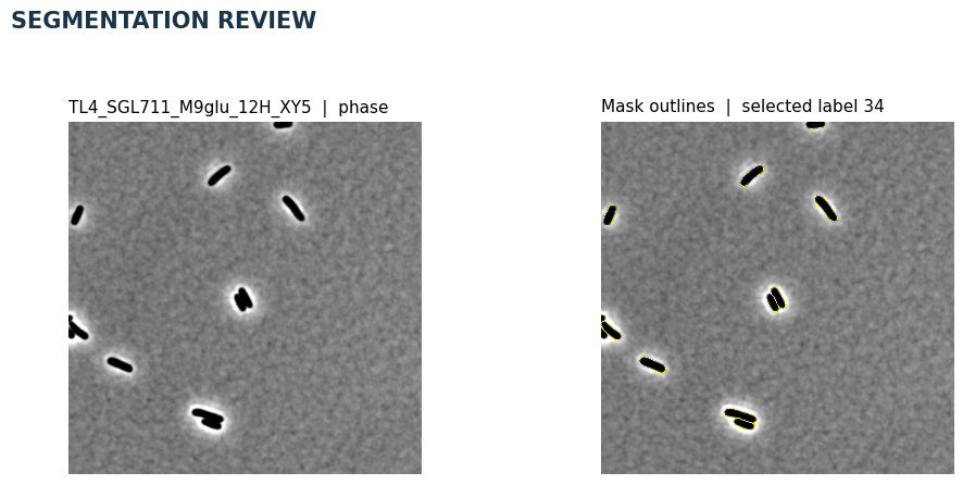
2. Segment and review. Saved notebook output from 3_channel_example; display settings are illustrative.
3. Build and inspect meshes
The mask becomes a cell contour, paired mesh sides, and a midline. join_thresh joins nearby poles in pixels; split_thresh controls splitting at constrictions; smoothing adjusts contour smoothness; CD_width selects the width-based constriction measure. save_data=True writes 3_channel_example_meshdata.pkl in RUN_DIR. Inspect the mesh on the phase image before loading fluorescence channels.
collection.batch_process_mesh(
    phase_channel=PHASE_CHANNEL, join_thresh=4, split_thresh=0.5,
    CD_width=False, smoothing=0.1, save_data=True,
)
print("Cells with meshes:", sum(len(image.cells) for image in collection.image_objects))
Optional: load saved meshes on a later run
If you already made meshes, skip the mesh-construction cell and run collection.batch_load_mesh("3_channel_example_meshdata.pkl", phase_channel=PHASE_CHANNEL) here. Keep the next inspection step.
# Uncomment on a later run after skipping mesh construction:
# collection.batch_load_mesh("3_channel_example_meshdata.pkl", phase_channel=PHASE_CHANNEL)
Choose a cell to inspect
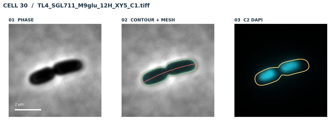
Set the field name and cell ID in the code cell below, then rerun it. The figure shows phase, contour, mesh, and midline; fluorescence is shown after object detection.
MESH_FIELD = "TL4_SGL711_M9glu_12H_XY5"
MESH_CELL_ID = 30
mesh_image, _ = bplt.select_example_cell(
    collection.image_objects, field_id=MESH_FIELD, cell_id=MESH_CELL_ID,
)
fig = bplt.plot_cell_gallery(mesh_image, MESH_CELL_ID, channel=None)
display(fig)
plt.close(fig)
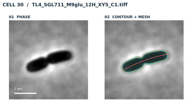
Choose a cell to inspect. Saved notebook output from 3_channel_example; display settings are illustrative.
4. Curate with the supplied SVM
DnaN_Timecourse.pkl is the model provided with this example. It uses morphology features to reject unsuitable meshes. Green outlines are retained and red outlines are rejected. save_curated_data=True writes 3_channel_example_curated_meshdata.pkl in RUN_DIR. Inspect the result before applying this model to other acquisitions; only load pickle files you trust.
#collection.batch_load_mesh("3_channel_example_meshdata.pkl", phase_channel=PHASE_CHANNEL)
before = bplt.snapshot_cell_contours(collection.image_objects)
before_count = sum(len(image.cells) for image in collection.image_objects)
collection.curate_dataset(str(MODEL_PATH), control=False, save_curated_data=True)
after_count = sum(len(image.cells) for image in collection.image_objects)
print(f"SVM curation: {before_count:,} to {after_count:,} cells")
fig = bplt.plot_curation_review(before, collection.image_objects
)
display(fig)
plt.close(fig)
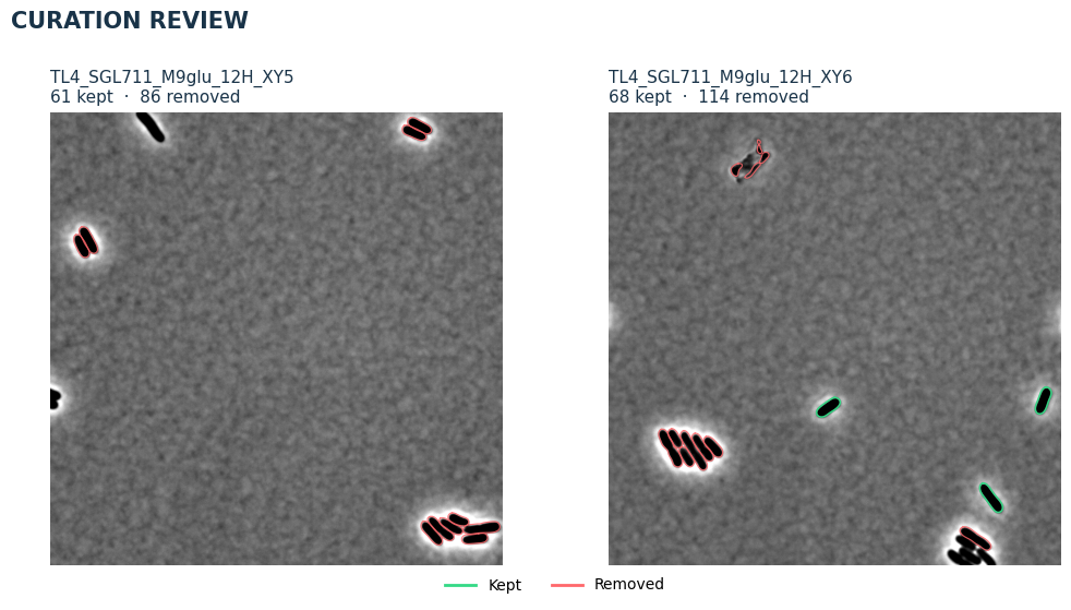
4. Curate with the supplied SVM. Saved notebook output from 3_channel_example; display settings are illustrative.
5. Detect GFP-DnaN objects
Object detection loads C3 and finds puncta inside curated cells. align=False leaves C3 in its original coordinates. Tune smoothing, log_sigma, kernel_width, and overlap limits for your images. The detected contours are stored on cells and later contribute to object features.
detections = collection.batch_detect_objects(
    channels=[DAPI,GFP_DNAN], reset_channels=True, align=False,
    smoothing=0.1, log_sigma=3, kernel_width=3,
    min_overlap_ratio=0.001, max_external_ratio=0.5,
)
print("Detected C3 objects:", len(detections))
collection.add_channels(collection.image_objects, [DAPI, GFP_DNAN])
Inspect a detected cell
Choose a curated field and cell ID directly below. The DAPI panel is cyan, GFP-DnaN is green, and the object outline shows what the detector found. If your chosen cell was removed by curation, pick an ID that remains in the green curation outlines.
OBJECT_FIELD = "TL4_SGL711_M9glu_12H_XY5"
OBJECT_CELL_ID = 62
object_image, _ = bplt.select_example_cell(
    collection.image_objects, field_id=OBJECT_FIELD, cell_id=OBJECT_CELL_ID,
)
fig = bplt.plot_cell_gallery(
    object_image,30, channel=DAPI, channel_label="DAPI",
)
display(fig)
plt.close(fig)
fig = bplt.plot_signal_gallery(
    object_image, 30,
    channel_labels={DAPI: "DAPI", GFP_DNAN: "GFP-DnaN"},
    show_objects=True,
)
display(fig)
plt.close(fig)
Inspect a detected cell. Saved notebook output from 3_channel_example; display settings are illustrative.
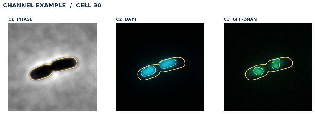
Inspect a detected cell. Saved notebook output from 3_channel_example; display settings are illustrative.
6. Extract features
channel_method_pairs assigns feature methods to channels. morphological measures cell geometry from the mesh; profiling measures each channel along the cell; objects summarizes C3 puncta. max_mesh_size excludes unusually large meshes. We compare the relative C3 object area fraction (C3_NC_ratio) with cell volume, avoiding an absolute fluorescence intensity comparison.
channel_method_pairs = [
    ([None], "morphological"),
    ([DAPI], "profiling"),
    ([GFP_DNAN], "profiling"),
    ([GFP_DNAN], "objects"),
]
collection.batch_calculate_features(
    channel_method_pairs, all_data=False, max_mesh_size=1000,
)
features = collection.merge_dataframes()
print(f"{len(features):,} cells x {len(features.columns)} columns")
display(features[["image_name", "cell_id", "cell_volume", "C3_NC_ratio"]].head())
7. Inspect relative measurements
C3_NC_ratio is the detected C3 object area divided by cell area. This comparison uses a within-cell fraction, so it does not require raw brightness to be comparable between fields.
fig, ax = plt.subplots(figsize=(5.5, 4))
valid = features[["cell_volume", "C3_NC_ratio"]].dropna()
ax.scatter(valid.cell_volume, valid.C3_NC_ratio,
           s=12, alpha=0.45, color="#31A85E")
ax.set(xlabel="Cell volume (um^3)", ylabel="C3 object area / cell area",
       title="GFP-DnaN object fraction vs cell volume")
fig.tight_layout()
display(fig)
plt.close(fig)
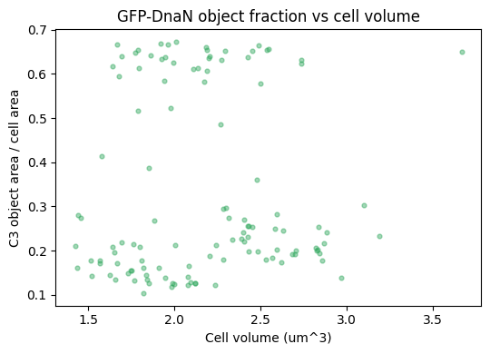
7. Inspect relative measurements. Saved notebook output from 3_channel_example; display settings are illustrative.
8. Save features and audit
dataframe_to_parquet() writes 3_channel_example_features.parquet; dataframe_to_pkl() writes 3_channel_example_features.pkl. Both go in RUN_DIR and contain one row per retained cell. A .pkl argument gives the exact pickle filename; a suffix without .pkl becomes a tag. Check processing_summary() for image and cell errors.
collection.dataframe_to_parquet()
pickle_path = collection.dataframe_to_pkl()
saved = pd.read_parquet(RUN_DIR / "3_channel_example_features.parquet")
summary = collection.processing_summary()
print("Saved Parquet and pickle:", len(saved), "rows;", pickle_path)
print("Image errors:", summary["error_count"],
      "Cell errors:", summary["cell_error_count"])